Socho tum ek company me kaam kar rahe ho.
Boss bolta hai:
"Employee experience badhne se salary kitni increase hoti hai?"
Ab har baar manually guess karna possible nahi hai. Yaha aata hai Linear Regression — ek simple but powerful ML technique jo relationship samajhta hai aur future predict karta hai.
1. Linear Regression kya hota hai?
Simple language me:
👉 Linear Regression ek technique hai jo input aur output ke beech ek straight line ka relation banata hai.
Example:
Input (X): Ad spend
Output (Y): Sales
Ye ek line banata hai:
"Agar X badhega, to Y kitna badhega"
Core Formula (sab kuch yahi hai)
y = mx + b
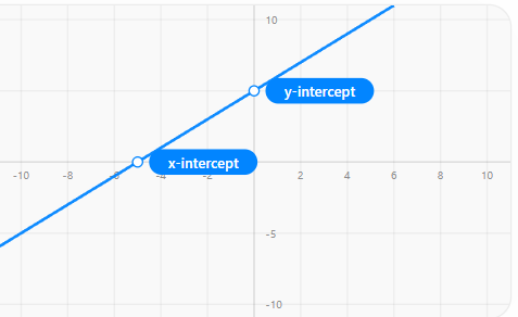
Iska matlab:
y = Output (prediction)
x = Input
m = slope (kitna change hoga)
b = intercept (jab x = 0 ho)
2. Real-Life Example
Ad Spend (₹) | Sales (₹) |
|---|---|
1000 | 5000 |
2000 | 7000 |
3000 | 9000 |
Model seekhega:
👉 "Har ₹1000 increase pe sales ₹2000 badh rahi hai"
To equation ban sakta hai:
Sales = 2 * AdSpend + 3000
3. Ye kaam kaise karta hai internally?
Step 1: Line guess karta hai
Random line banata hai.
Step 2: Error calculate karta hai
Error = Actual value - Predicted value
Step 3: Cost Function use karta hai
👉 Most common: Mean Squared Error (MSE)
Formula (simple me):
Error^2 ka average
Step 4: Gradient Descent
👉 Model dheere-dheere line ko adjust karta hai taki error kam ho jaye.
4. Gradient Descent kya hota hai?
Socho tum pahad se neeche utar rahe ho and goal hai lowest point.
👉 Har step me tum neeche ki taraf move karte ho
Waise hi:
Model slope aur intercept adjust karta hai
Jab tak error minimum na ho jaye
5. Types of Linear Regression
1. Simple Linear Regression
👉 Ek input, ek output
Example:
Experience → Salary
2. Multiple Linear Regression
👉 Multiple inputs
Example:
Experience + Skills + Location → Salary
Formula:
y = m1x1 + m2x2 + m3x3 + b
6. Real Industry Use Cases
Sales Forecasting
Ads vs Sales prediction
Banking
Loan amount vs risk
Real Estate
Area + Location → Price
HR Analytics
Experience + Performance → Salary
7. Important Concepts
1. Residuals
Actual - Predicted difference
2. R² Score (Accuracy measure)
0 → bekar model
1 → perfect model
Example:
R² = 0.85 → 85% data explain ho raha hai
3. Assumptions (bahut important)
Linear Regression tab best kaam karta hai jab:
Relationship linear ho
Errors random ho
Data independent ho
Variance constant ho
8. Where Linear Regression FAILS
Non-linear data
Example:
Age vs Happiness (straight line nahi hoti)
Outliers
Ek extreme value pura model bigaad deta hai
Multicollinearity
Inputs ek dusre se heavily related ho
9. Practical Workflow
Step-by-step:
Data collect karo
Data clean karo (null, outliers)
Visualisation karo (scatter plot)
Train-test split
Model train karo
Predictions lo
Evaluate karo (R², MSE)
Deploy karo (API / dashboard)
10. Python Example (Simple)
from sklearn.linear_model import LinearRegression

model = LinearRegression()
model.fit(X_train, y_train)

y_pred = model.predict(X_test)
Next Steps:-
Agar tumne ye samajh liya, next learn karo:
Polynomial Regression
Ridge & Lasso Regression
Logistic Regression (classification)
Feature Engineering
Real datasets pe practice (Kaggle)
Linear Regression Project (Ad Spend → Sales)
# ==============================
# 1. Import Required Libraries
# ==============================

import pandas as pd                      # data handle karne ke liye
import numpy as np                       # numerical operations ke liye
import matplotlib.pyplot as plt          # visualization ke liye

from sklearn.model_selection import train_test_split   # train-test split
from sklearn.linear_model import LinearRegression      # model
from sklearn.metrics import mean_squared_error, r2_score  # evaluation


# ==============================
# 2. Load Dataset
# ==============================

# CSV file read kar rahe hain (apna path change karna)
data = pd.read_csv("ads_data.csv")

# First 5 rows dekhne ke liye
print(data.head())


# ==============================
# 3. Basic Data Understanding
# ==============================

print(data.info())        # columns, datatype check
print(data.describe())    # statistical summary


# ==============================
# 4. Data Cleaning
# ==============================

# null values check
print(data.isnull().sum())

# simple approach: null rows hata do
data = data.dropna()

# NOTE:
# real project me median/mean se fill karte hain


# ==============================
# 5. Data Visualization
# ==============================

# TV Ads vs Sales ka relation check
plt.scatter(data['TV Ads'], data['Sales'])
plt.xlabel("TV Ads Spend")
plt.ylabel("Sales")
plt.title("TV Ads vs Sales")
plt.show()

# NOTE:
# yaha dekhte hain relation linear hai ya nahi


# ==============================
# 6. Feature Selection
# ==============================

# Input features (independent variables)
X = data[['TV Ads', 'Facebook Ads', 'Google Ads']]

# Output (dependent variable)
y = data['Sales']


# ==============================
# 7. Train-Test Split
# ==============================

# 80% training, 20% testing
X_train, X_test, y_train, y_test = train_test_split(
    X, y, test_size=0.2, random_state=42
)

# random_state fix karne se same result aata hai har run me


# ==============================
# 8. Model Training
# ==============================

model = LinearRegression()     # model object create
model.fit(X_train, y_train)    # training


# ==============================
# 9. Prediction
# ==============================

y_pred = model.predict(X_test)

# predicted vs actual compare kar sakte ho
print("Predictions:", y_pred[:5])
print("Actual:", y_test.values[:5])


# ==============================
# 10. Model Evaluation
# ==============================

mse = mean_squared_error(y_test, y_pred)
r2 = r2_score(y_test, y_pred)

print("Mean Squared Error:", mse)
print("R2 Score:", r2)

# MSE kam hona chahiye
# R2 1 ke paas hona chahiye


# ==============================
# 11. Model Coefficients (Insight)
# ==============================

print("Coefficients:", model.coef_)
print("Intercept:", model.intercept_)

# iska matlab:
# har feature ka impact kya hai


# ==============================
# 12. Custom Prediction (Real Use)
# ==============================

# Example: new ad budget
# TV = 2000, Facebook = 500, Google = 300

new_data = [[2000, 500, 300]]

prediction = model.predict(new_data)

print("Predicted Sales:", prediction)

# NOTE:
# real project me yahi API ya dashboard me use hota hai


# ==============================
# 13. (Optional) Save Model
# ==============================

import joblib

joblib.dump(model, "linear_regression_model.pkl")

# baad me load karne ke liye:
# model = joblib.load("linear_regression_model.pkl")