1. Introduction — What is NumPy and Why Should You Care? {introduction}
NumPy stands for Numerical Python. It is the foundation of almost every data science and scientific computing library in Python — pandas, scikit-learn, TensorFlow, OpenCV — they all use NumPy under the hood.
The Core Problem NumPy Solves
# Python list — slow, no vectorization
python_list = [1, 2, 3, 4, 5]
result = [x * 2 for x in python_list]  # Loop needed — slow!

# NumPy array — fast, vectorized
import numpy as np
numpy_array = np.array([1, 2, 3, 4, 5])
result = numpy_array * 2  # No loop needed — blazing fast!
Why is NumPy So Fast?
Written in C and Fortran under the hood
Uses contiguous memory blocks (not scattered like Python lists)
Leverages SIMD (Single Instruction Multiple Data) — CPU-level parallelism
Avoids Python's interpreter overhead via vectorized operations
Real-World Usage
Domain | How NumPy is Used |
|---|---|
Data Science | Array math, feature engineering |
Machine Learning | Matrix operations, weight updates |
Image Processing | Images are 3D arrays (H × W × Channels) |
Financial Analysis | Time series, portfolio math |
Signal Processing | FFT, filters, waveform analysis |
Physics Simulations | N-body problems, fluid dynamics |
NumPy vs Python List — Speed Comparison
import numpy as np
import time

# 10 million elements
size = 10_000_000

# Python list
py_list = list(range(size))
start = time.time()
result = [x * 2 for x in py_list]
print(f"Python list: {time.time() - start:.3f}s")
# Output: Python list: 0.847s

# NumPy array
np_arr = np.arange(size)
start = time.time()
result = np_arr * 2
print(f"NumPy array: {time.time() - start:.3f}s")
# Output: NumPy array: 0.011s
# NumPy is ~75x faster!
2. Installation & Setup {#installation}
# Install NumPy
pip install numpy

# With Anaconda (recommended for data science)
conda install numpy

# Check version
python -c "import numpy as np; print(np.__version__)"
Standard Import Convention
import numpy as np # Always use 'np' alias — universal convention
3. The Core — ndarray (N-Dimensional Array)
The ndarray is NumPy's primary object. Think of it as a grid of values, all of the same data type, stored in a contiguous block of memory.
Understanding Dimensions
import numpy as np
# 0D Array — Scalar
scalar = np.array(42)
print(scalar.ndim) # 0
print(scalar.shape) # ()
# 1D Array — Vector (like a spreadsheet row)
vector = np.array([1, 2, 3, 4, 5])
print(vector.ndim) # 1
print(vector.shape) # (5,)
# 2D Array — Matrix (like a spreadsheet / DataFrame)
matrix = np.array([[1, 2, 3],
[4, 5, 6]])
print(matrix.ndim) # 2
print(matrix.shape) # (2, 3) — 2 rows, 3 columns
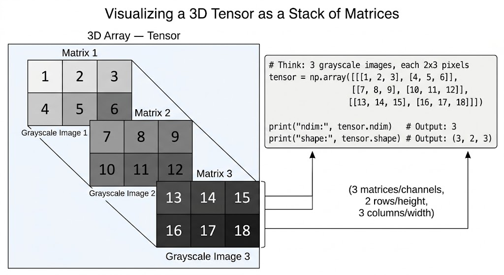
# 3D Array — Tensor (like a stack of matrices)
# Think: 3 grayscale images, each 2x3 pixels
tensor = np.array([[[1, 2, 3],
[4, 5, 6]],
[[7, 8, 9],
[10, 11, 12]],
[[13, 14, 15],
[16, 17, 18]]])
print(tensor.ndim) # 3
print(tensor.shape) # (3, 2, 3)
Real-World Dimension Analogy
Dimensions | Shape Example | Real-World Analogy |
|---|---|---|
0D |
| Single number: 3.14 |
1D |
| One row of data |
2D |
| DataFrame: 100 rows, 5 columns |
3D |
| Color image: 3 channels (RGB), 224×224 pixels |
4D |
| Batch of 32 color images |
4. NumPy Data Types (dtype)
NumPy arrays are homogeneous — all elements must be the same type. This is why they're so fast.
Complete dtype Reference
import numpy as np

# Integer types
a = np.array([1, 2, 3], dtype=np.int8)    # -128 to 127
b = np.array([1, 2, 3], dtype=np.int16)   # -32,768 to 32,767
c = np.array([1, 2, 3], dtype=np.int32)   # ~-2 billion to 2 billion
d = np.array([1, 2, 3], dtype=np.int64)   # Very large integers

# Unsigned integers (no negatives — saves memory)
e = np.array([1, 2, 3], dtype=np.uint8)   # 0 to 255 (pixel values!)
f = np.array([1, 2, 3], dtype=np.uint32)  # 0 to ~4 billion

# Float types
g = np.array([1.0], dtype=np.float16)     # Half precision — ML on GPU
h = np.array([1.0], dtype=np.float32)     # Single precision — ML standard
i = np.array([1.0], dtype=np.float64)     # Double precision — default
j = np.array([1.0], dtype=np.float128)    # Quad precision (not on Windows)

# Complex numbers
k = np.array([1+2j, 3+4j], dtype=np.complex64)
l = np.array([1+2j, 3+4j], dtype=np.complex128)

# Boolean
m = np.array([True, False, True], dtype=np.bool_)

# String (fixed-width)
n = np.array(['Alice', 'Bob', 'Charlie'], dtype=np.str_)

# Checking dtype
print(d.dtype)          # int64
print(d.itemsize)       # 8 bytes per element
print(d.nbytes)         # total bytes in array
dtype Inference & Type Casting
import numpy as np

# NumPy infers dtype automatically
arr1 = np.array([1, 2, 3])         # int64 (default int)
arr2 = np.array([1.0, 2.0, 3.0])  # float64 (default float)
arr3 = np.array([1, 2.5, 3])      # float64 (upcasts to float!)
arr4 = np.array([True, False])     # bool_

# Manual type casting
arr = np.array([1.7, 2.9, 3.1])
int_arr = arr.astype(np.int32)     # [1, 2, 3] — truncates, not rounds!
print(int_arr)

# Safe casting check
print(np.can_cast(np.float64, np.int32))  # False — lossy!
print(np.can_cast(np.int32, np.float64))  # True — safe

# Memory optimization tip
# Default int64 vs int8 for small values
big = np.array([1, 2, 3], dtype=np.int64)
small = np.array([1, 2, 3], dtype=np.int8)
print(big.nbytes)    # 24 bytes
print(small.nbytes)  # 3 bytes  — 8x smaller!
When to Use Which dtype?
Use Case | Recommended dtype |
|---|---|
Pixel values (0–255) |
|
ML model weights |
|
Financial calculations |
|
Age / small integers |
|
Large IDs |
|
True/False masks |
|
GPU-based deep learning |
|
5. Array Creation — All Methods Explained
From Python Data Structures
import numpy as np

# From list
arr = np.array([1, 2, 3, 4, 5])

# From tuple
arr = np.array((10, 20, 30))

# From list of lists (2D)
matrix = np.array([[1, 2, 3], [4, 5, 6]])

# From range
arr = np.array(range(10))  # Works but np.arange is better
Built-in Initialization Functions
import numpy as np

# --- ZEROS & ONES ---
zeros = np.zeros(5)                     # [0. 0. 0. 0. 0.]
zeros_2d = np.zeros((3, 4))            # 3x4 matrix of zeros
ones = np.ones((2, 3), dtype=np.int32) # 2x3 matrix of integer 1s
full = np.full((3, 3), 7)              # 3x3 matrix filled with 7
full_like = np.full_like(zeros_2d, 9)  # Same shape as zeros_2d, filled with 9

# --- IDENTITY & EYE ---
identity = np.eye(4)          # 4x4 identity matrix (diagonal = 1)
eye_k = np.eye(4, k=1)       # k=1: diagonal shifted up by 1
diag = np.diag([1, 2, 3, 4]) # Diagonal matrix from array

# --- RANGES ---
# np.arange(start, stop, step) — like Python range() but returns array
arange = np.arange(0, 10, 2)          # [0 2 4 6 8]
arange_f = np.arange(0.0, 1.0, 0.25) # [0.   0.25 0.5  0.75]

# np.linspace(start, stop, num) — num evenly spaced points INCLUDING stop
linspace = np.linspace(0, 1, 5)       # [0.   0.25 0.5  0.75 1.  ]
linspace_excl = np.linspace(0, 1, 5, endpoint=False)  # Excludes stop

# np.logspace(start, stop, num) — logarithmically spaced
logspace = np.logspace(0, 3, 4)       # [1. 10. 100. 1000.]

# np.geomspace — geometric spacing
geomspace = np.geomspace(1, 1000, 4)  # [1. 10. 100. 1000.]

# --- RANDOM ARRAYS ---
np.random.seed(42)                          # For reproducibility!
rand_uniform = np.random.rand(3, 4)         # Uniform [0, 1)
rand_normal = np.random.randn(3, 4)         # Standard normal (mean=0, std=1)
rand_int = np.random.randint(0, 100, (3,4)) # Random integers [0, 100)
rand_choice = np.random.choice([10,20,30,40], size=5, replace=True)
rand_shuffle = np.arange(10)
np.random.shuffle(rand_shuffle)             # In-place shuffle

# New recommended random API (NumPy 1.17+)
rng = np.random.default_rng(seed=42)
arr = rng.random((3, 4))           # Better randomness than np.random.rand
arr = rng.integers(0, 100, (3,4)) # Better than np.random.randint
arr = rng.normal(loc=0, scale=1, size=(3,4))

# --- EMPTY (Uninitialized — Fastest but Dangerous!) ---
empty = np.empty((3, 4))   # Contains garbage values! Use only if you'll fill it
empty_like = np.empty_like(zeros_2d)

# --- FROM FUNCTIONS ---
# np.fromfunction — create array by applying function to indices
arr = np.fromfunction(lambda i, j: i + j, (4, 4), dtype=int)
# [[0 1 2 3]
#  [1 2 3 4]
#  [2 3 4 5]
#  [3 4 5 6]]

# np.fromiter — create from iterator
arr = np.fromiter((x**2 for x in range(5)), dtype=float)  # [0. 1. 4. 9. 16.]
Copying Arrays — Deep vs Shallow
import numpy as np
original = np.array([1, 2, 3, 4, 5])

# VIEW — shares memory (no copy!)
view = original[2:5]        # This is a VIEW
view[0] = 99                # Modifies original too!
print(original)             # [1 2 99 4 5] ← changed!

# COPY — independent
copy = original.copy()
copy[0] = 999
print(original)             # [1 2 99 4 5] ← unchanged
print(copy)                 # [999 2 99 4 5]

# Check if an array owns its data
print(view.base is original)  # True — it's a view
print(copy.base is None)      # True — it owns its data
⚠️ Critical Rule: Slicing creates a view, not a copy. This catches many beginners off guard. Use
.copy()explicitly when you need independent data.
6. Array Attributes — Shape, Size, Ndim, Strides {#attributes}
import numpy as np

arr = np.array([[1, 2, 3, 4],
                [5, 6, 7, 8],
                [9, 10, 11, 12]])

print(arr.ndim)     # 2 — number of dimensions
print(arr.shape)    # (3, 4) — (rows, columns)
print(arr.size)     # 12 — total number of elements
print(arr.dtype)    # int64
print(arr.itemsize) # 8 — bytes per element
print(arr.nbytes)   # 96 — total bytes (12 × 8)

# Strides — bytes to step in each dimension
print(arr.strides)  # (32, 8) — 32 bytes to next row, 8 bytes to next col
# Because: 4 columns × 8 bytes/element = 32 bytes per row

# T — transpose
print(arr.T)        # (4, 3) — rows and columns swapped
print(arr.T.shape)  # (4, 3)

# flat — 1D iterator over all elements
for x in arr.flat:
    print(x, end=' ')  # 1 2 3 4 5 6 7 8 9 10 11 12
7. Indexing — Accessing Array Elements {#indexing}
1D Indexing
import numpy as np

arr = np.array([10, 20, 30, 40, 50])

# Positive indexing
print(arr[0])   # 10 — first element
print(arr[4])   # 50 — last via index
print(arr[-1])  # 50 — last via negative
print(arr[-2])  # 40 — second from last

# Modifying elements
arr[0] = 99
print(arr)   # [99 20 30 40 50]
2D Indexing
import numpy as np

matrix = np.array([[1, 2, 3],
                   [4, 5, 6],
                   [7, 8, 9]])

# Single element — [row, column]
print(matrix[0, 0])   # 1  — top-left
print(matrix[1, 2])   # 6  — row 1, col 2
print(matrix[-1, -1]) # 9  — bottom-right

# Entire row
print(matrix[0])      # [1 2 3]
print(matrix[0, :])   # [1 2 3] — same thing

# Entire column
print(matrix[:, 1])   # [2 5 8] — column 1

# Submatrix
print(matrix[0:2, 1:3])  # [[2 3] [5 6]]
3D Indexing
import numpy as np

# Imagine: 2 grayscale images, each 3x3 pixels
tensor = np.arange(18).reshape(2, 3, 3)
# [[[ 0  1  2]
#   [ 3  4  5]
#   [ 6  7  8]]
#  [[ 9 10 11]
#   [12 13 14]
#   [15 16 17]]]

print(tensor[0])       # First image (3x3)
print(tensor[0, 1])    # First image, second row: [3 4 5]
print(tensor[0, 1, 2]) # First image, row 1, col 2: 5
print(tensor[:, 0, :]) # First row of BOTH images
8. Slicing — Extracting Sub-Arrays {#slicing}
Slice Syntax: [start:stop:step]
import numpy as np

arr = np.array([0, 10, 20, 30, 40, 50, 60, 70, 80, 90])

# Basic slicing
print(arr[2:5])     # [20 30 40] — index 2, 3, 4
print(arr[:4])      # [0 10 20 30] — start to index 3
print(arr[6:])      # [60 70 80 90] — index 6 to end
print(arr[:])       # All elements

# Step
print(arr[::2])     # [0 20 40 60 80] — every 2nd
print(arr[1::2])    # [10 30 50 70 90] — odd indices
print(arr[::-1])    # [90 80 70 60 50 40 30 20 10 0] — REVERSE!
print(arr[::-2])    # [90 70 50 30 10] — reverse every 2nd

# 2D slicing
matrix = np.arange(1, 26).reshape(5, 5)
# [[ 1  2  3  4  5]
#  [ 6  7  8  9 10]
#  [11 12 13 14 15]
#  [16 17 18 19 20]
#  [21 22 23 24 25]]

print(matrix[1:4, 1:4])
# [[ 7  8  9]
#  [12 13 14]
#  [17 18 19]]

print(matrix[::2, ::2])
# [[ 1  3  5]
#  [11 13 15]
#  [21 23 25]]

# Real use case: downsample an image by taking every 2nd pixel
# downsampled = image[::2, ::2]  — halves resolution
9. Fancy Indexing & Boolean Indexing {#fancy-indexing}
Fancy Indexing — Index with Arrays
import numpy as np

arr = np.array([10, 20, 30, 40, 50, 60])

# Index with a list of indices
indices = [0, 2, 5]
print(arr[indices])    # [10 30 60]

# 2D fancy indexing
matrix = np.arange(12).reshape(4, 3)
# [[ 0  1  2]
#  [ 3  4  5]
#  [ 6  7  8]
#  [ 9 10 11]]

rows = [0, 2, 3]
cols = [1, 0, 2]
print(matrix[rows, cols])  # [1 6 11] — pairs: (0,1), (2,0), (3,2)

# Select specific rows
print(matrix[[0, 3]])    # Rows 0 and 3

# Use case: select top-k predicted classes in ML
scores = np.array([0.1, 0.8, 0.05, 0.9, 0.3])
top_k_indices = np.argsort(scores)[-3:][::-1]  # Indices of top 3
print(top_k_indices)      # [3 1 4]
print(scores[top_k_indices])  # [0.9 0.8 0.3]
Boolean Indexing — Filter with Conditions
import numpy as np

arr = np.array([5, 15, 25, 35, 45, 55])

# Create boolean mask
mask = arr > 20
print(mask)       # [False False  True  True  True  True]

# Apply mask
print(arr[mask])  # [25 35 45 55]

# Inline — most common pattern
print(arr[arr > 20])         # [25 35 45 55]
print(arr[arr % 10 == 5])    # [5 15 25 35 45 55] — all have 5 in units

# Multiple conditions
print(arr[(arr > 10) & (arr < 50)])   # [15 25 35 45]
print(arr[(arr < 10) | (arr > 50)])   # [5 55]
print(arr[~(arr > 30)])               # [5 15 25 30] — NOT greater than 30

# 2D boolean indexing
matrix = np.arange(1, 13).reshape(3, 4)
print(matrix[matrix % 2 == 0])  # [2 4 6 8 10 12] — all even elements, flattened!

# Real-world: replace outliers with median
data = np.array([12.5, 13.1, 999.9, 12.8, 13.0, -500.0, 12.9])
median = np.median(data)
data[np.abs(data - median) > 100] = median  # Replace outliers
print(data)

# np.where — conditional selection
x = np.array([1, -2, 3, -4, 5])
result = np.where(x > 0, x, 0)  # If positive keep it, else replace with 0
print(result)  # [1 0 3 0 5]

# np.where with two arrays
a = np.array([1, 2, 3, 4, 5])
b = np.array([10, 20, 30, 40, 50])
condition = np.array([True, False, True, False, True])
result = np.where(condition, a, b)  # [1 20 3 40 5]
10. Array Manipulation — Reshape, Resize, Flatten, Ravel {#manipulation}
import numpy as np

arr = np.arange(12)  # [0 1 2 3 4 5 6 7 8 9 10 11]

# --- RESHAPE ---
# Returns a VIEW (if possible), same data, different shape
reshaped = arr.reshape(3, 4)     # 3 rows, 4 cols
reshaped = arr.reshape(2, 2, 3)  # 3D: 2×2×3
reshaped = arr.reshape(3, -1)    # -1 means "figure it out" → (3, 4)
reshaped = arr.reshape(-1, 4)    # → (3, 4)
reshaped = arr.reshape(1, -1)    # Row vector: (1, 12)
reshaped = arr.reshape(-1, 1)    # Column vector: (12, 1)

# --- RESIZE ---
# Modifies array IN-PLACE, fills with repeated data if larger
arr2 = np.array([1, 2, 3])
arr2.resize(5)           # [1 2 3 1 2] — repeats!
np.resize(arr2, (2, 3)) # Returns new array, repeats data

# --- FLATTEN vs RAVEL ---
matrix = np.array([[1, 2, 3], [4, 5, 6]])

flat = matrix.flatten()  # Always returns a COPY — safe to modify
ravel = matrix.ravel()   # Returns a VIEW if possible — faster but careful!

flat[0] = 99
print(matrix[0, 0])  # 1 — original unchanged (flatten is a copy)

ravel[0] = 99
print(matrix[0, 0])  # 99 — original changed! (ravel is a view)

# --- TRANSPOSE ---
arr = np.arange(6).reshape(2, 3)
# [[0 1 2]
#  [3 4 5]]
print(arr.T)         # [[0 3] [1 4] [2 5]] — shape (3, 2)
print(arr.T.shape)   # (3, 2)

# For higher dimensions — np.transpose with axes
arr_3d = np.arange(24).reshape(2, 3, 4)
transposed = np.transpose(arr_3d, axes=(0, 2, 1))
print(transposed.shape)  # (2, 4, 3)

# --- SQUEEZE & EXPAND_DIMS ---
arr = np.array([[[1, 2, 3]]])  # Shape: (1, 1, 3)
squeezed = np.squeeze(arr)     # Shape: (3,) — removes all size-1 dimensions
squeezed = np.squeeze(arr, axis=0)  # Shape: (1, 3) — remove only axis 0

arr = np.array([1, 2, 3])     # Shape: (3,)
expanded = np.expand_dims(arr, axis=0)  # Shape: (1, 3) — add row dimension
expanded = np.expand_dims(arr, axis=1)  # Shape: (3, 1) — add column dimension

# The newaxis trick (same as expand_dims)
print(arr[np.newaxis, :].shape)  # (1, 3)
print(arr[:, np.newaxis].shape)  # (3, 1)
Stacking & Splitting
import numpy as np

a = np.array([1, 2, 3])
b = np.array([4, 5, 6])

# --- STACKING ---
np.vstack([a, b])   # Vertical stack → [[1 2 3] [4 5 6]] shape (2,3)
np.hstack([a, b])   # Horizontal stack → [1 2 3 4 5 6] shape (6,)
np.stack([a, b])    # New axis → [[1 2 3] [4 5 6]] shape (2,3)
np.stack([a, b], axis=1)  # → [[1 4] [2 5] [3 6]] shape (3,2)
np.concatenate([a, b])    # → [1 2 3 4 5 6] — join along existing axis
np.column_stack([a, b])   # → [[1 4] [2 5] [3 6]] — like stack axis=1

# 2D stacking
m1 = np.array([[1, 2], [3, 4]])
m2 = np.array([[5, 6], [7, 8]])
np.vstack([m1, m2])         # Shape (4, 2) — stack rows
np.hstack([m1, m2])         # Shape (2, 4) — stack columns
np.concatenate([m1, m2], axis=0)  # Same as vstack
np.concatenate([m1, m2], axis=1)  # Same as hstack

# --- SPLITTING ---
arr = np.arange(12)

np.split(arr, 3)            # Split into 3 equal parts → [0-3], [4-7], [8-11]
np.split(arr, [3, 7])       # Split at index 3 and 7 → [0-2], [3-6], [7-11]
np.array_split(arr, 5)      # 5 parts, unequal OK (no error)

matrix = np.arange(16).reshape(4, 4)
np.vsplit(matrix, 2)        # Split into 2 parts vertically (by rows)
np.hsplit(matrix, 2)        # Split into 2 parts horizontally (by cols)
11. Broadcasting — The Secret Superpower {#broadcasting}
Broadcasting is how NumPy handles arithmetic between arrays of different shapes without making copies.
Broadcasting Rules
If arrays have different ndim, the smaller shape is padded with 1s on the left
Dimensions with size 1 are stretched to match the other
If shapes are still incompatible →
ValueError
import numpy as np

# Rule: shape (3,) vs shape (3,) → simple math
a = np.array([1, 2, 3])
b = np.array([10, 20, 30])
print(a + b)  # [11 22 33]

# Shape (3,) vs scalar — scalar broadcasts to (3,)
print(a + 100)  # [101 102 103]
print(a * 2)    # [2 4 6]

# Shape (3, 1) vs (1, 4) → result is (3, 4)
col = np.array([[1], [2], [3]])    # shape (3, 1)
row = np.array([[10, 20, 30, 40]]) # shape (1, 4)
print(col + row)
# [[11 21 31 41]
#  [12 22 32 42]
#  [13 23 33 43]]

# Shape (3,) vs (4, 3) — works! (3,) becomes (1, 3) then (4, 3)
matrix = np.arange(12).reshape(4, 3)
bias = np.array([10, 20, 30])
result = matrix + bias  # Add bias to each row
print(result)

# Real ML use case: normalize each feature column
data = np.array([[1, 200, 3000],
                 [2, 400, 6000],
                 [3, 600, 9000]])
mean = data.mean(axis=0)  # Mean of each column: [2, 400, 6000]
std = data.std(axis=0)    # Std of each column
normalized = (data - mean) / std  # Broadcasting! mean and std shape (3,)
print(normalized)
Broadcasting Failures
import numpy as np

a = np.array([[1, 2, 3], [4, 5, 6]])  # shape (2, 3)
b = np.array([1, 2])                   # shape (2,)

# This FAILS — (2,3) vs (2,) — trailing dims don't match
try:
    print(a + b)
except ValueError as e:
    print(e)  # operands could not be broadcast together with shapes (2,3) (2,)

# FIX: reshape b to (2, 1) — column vector
b_fixed = b[:, np.newaxis]  # shape (2, 1)
print(a + b_fixed)
# [[2 3 4]
#  [6 7 8]]
12. Edge Cases & Common Errors {#errors}
Error 1: View vs Copy Confusion
import numpy as np

arr = np.arange(10)
# WRONG — thinking this is a copy
sub = arr[2:5]
sub[0] = 999
print(arr)  # [0 1 999 3 4 5 6 7 8 9] — modified original!

# CORRECT
sub = arr[2:5].copy()  # Always call .copy() if you need independence
Error 2: Shape Mismatch in Operations
import numpy as np
a = np.array([[1, 2, 3]])  # shape (1, 3)
b = np.array([[1], [2]])   # shape (2, 1)
# a + b → (2, 3) — works via broadcasting

a = np.array([1, 2, 3])   # shape (3,)
b = np.array([1, 2])      # shape (2,)
# a + b → ValueError! shapes don't broadcast
Error 3: Integer Division Truncation
import numpy as np
arr = np.array([1, 2, 3], dtype=np.int32)
print(arr / 2)   # [0.5 1.  1.5] — returns float64 (Python 3)
print(arr // 2)  # [0 1 1] — integer floor division
print(arr.astype(float) / 2)  # Explicit float division
Error 4: np.nan in Integer Arrays
import numpy as np
# This FAILS — int can't hold NaN
arr = np.array([1, 2, np.nan], dtype=np.int32)  # ValueError!

# SOLUTION — use float
arr = np.array([1, 2, np.nan], dtype=np.float64)  # Works

# pandas nullable integers solve this with Int32 dtype (capital I)
Error 5: Modifying Array During Iteration
import numpy as np
arr = np.array([1, 2, 3, 4, 5])

# WRONG — don't modify while iterating
for i, val in enumerate(arr):
    if val % 2 == 0:
        arr = np.delete(arr, i)  # Unpredictable!

# CORRECT — use boolean indexing
arr = arr[arr % 2 != 0]  # [1 3 5]
Error 6: Comparing Floats
import numpy as np
# WRONG
a = np.float64(0.1 + 0.2)
print(a == 0.3)  # False! Floating point precision issue

# CORRECT
print(np.isclose(a, 0.3))              # True
print(np.allclose(arr1, arr2))         # For entire arrays
print(np.isclose(a, 0.3, atol=1e-8))  # Custom tolerance
13. Pro Tips for Part 1 {#pro-tips}
Memory Layout: C-order vs Fortran-order
import numpy as np

# C-order (row-major) — default — row elements are contiguous
arr_c = np.array([[1,2,3],[4,5,6]], order='C')

# Fortran-order (column-major) — column elements are contiguous
arr_f = np.array([[1,2,3],[4,5,6]], order='F')

# Row iteration is faster in C-order, column iteration in F-order
# Use C-order for row-wise operations (most common)
# Use F-order for column-wise operations (LAPACK/BLAS compatibility)
print(arr_c.flags['C_CONTIGUOUS'])  # True
print(arr_f.flags['F_CONTIGUOUS'])  # True
Memory-Efficient Patterns
import numpy as np

# DON'T create unnecessary copies
# BAD
result = np.array([x * 2 for x in arr])  # Creates a list first, then array

# GOOD
result = arr * 2  # Pure NumPy — no intermediate list

# In-place operations save memory
arr += 10        # Modifies in-place, no new allocation
arr *= 2         # vs arr = arr * 2 which creates new array

# Pre-allocate when building arrays iteratively
# BAD
result = np.array([])
for i in range(1000):
    result = np.append(result, i)  # O(n²) — very slow!

# GOOD
result = np.empty(1000)
for i in range(1000):
    result[i] = i  # O(n) — fast

# BEST
result = np.arange(1000)  # Even better — no loop at all
Using np.einsum for Complex Operations
import numpy as np

# Einsum — Einstein summation convention
# Can express dot products, outer products, traces, transposes, etc.
A = np.random.rand(3, 4)
B = np.random.rand(4, 5)

# Matrix multiplication
C = np.einsum('ij,jk->ik', A, B)  # Same as A @ B

# Batch matrix multiplication (useful in deep learning)
batch_A = np.random.rand(10, 3, 4)  # 10 matrices of shape 3×4
batch_B = np.random.rand(10, 4, 5)  # 10 matrices of shape 4×5
result = np.einsum('bij,bjk->bik', batch_A, batch_B)  # (10, 3, 5)

# Trace of a matrix
A = np.random.rand(4, 4)
trace = np.einsum('ii->', A)  # Same as np.trace(A)
14. Interview Questions — Part 1 {#interview}
Basic Level
Q1: What is NumPy? Why is it faster than Python lists?
NumPy is a numerical computing library. It's faster because it stores data in contiguous memory, uses C/Fortran compiled code, and supports vectorized operations (no Python interpreter loop).
Q2: What is ndarray? How is it different from a Python list?
ndarray is a multidimensional, fixed-type array. Unlike lists: all elements must be same type, stored contiguously in memory, supports vectorized math.
Q3: What is the difference between shape and size?
shapeis a tuple of dimensions:(3, 4).sizeis total elements:12.
Q4: What happens when you add an int32 and float64 NumPy array?
NumPy upcasts to the higher precision type (float64) — same as C language promotion rules.
Intermediate Level
Q5: What is the difference between flatten() and ravel()?
flatten()always returns a copy.ravel()returns a view if possible, copy if not.ravel()is faster but modifying it may affect the original array.
Q6: Explain broadcasting with an example.
Broadcasting allows NumPy to perform element-wise operations on arrays with different shapes by virtually stretching the smaller array. E.g., adding shape
(3,)to shape(4, 3)— the(3,)is treated as(1, 3)then stretched to(4, 3).
Q7: What is the difference between a view and a copy in NumPy? How do you check?
View shares data with original (changes affect both). Copy is independent. Check with
arr.base— if notNone, it's a view. Or usenp.shares_memory(a, b).
Q8: When would you use np.empty() instead of np.zeros()?
When you plan to fill every element before reading it.
np.empty()skips initialization so it's faster, but contains garbage values.
Advanced Level
Q9: What are strides in NumPy?
Strides are the number of bytes to step in each dimension when traversing an array. For shape
(3, 4)withint64: strides are(32, 8)— 32 bytes to next row, 8 bytes to next column. NumPy'sreshapeworks by changing strides, not copying data.
Q10: How does NumPy implement transpose without copying data?
By swapping the strides tuple. A
(3, 4)array with strides(32, 8)becomes(4, 3)with strides(8, 32)— same data, different traversal order.
Scenario-Based
Q11: You have a 1M element array. How would you efficiently replace all negative values with 0?
arr[arr < 0] = 0  # Boolean indexing — vectorized, no loop
# Or
arr = np.maximum(arr, 0)  # Slightly faster — no boolean mask creation
Q12: How would you select every other row from a 2D array?
matrix[::2] # Slicing with step 2
End of Part 1 — Foundations & Arrays
Up Next → Part 2: Mathematical Operations, Statistical Functions, Linear Algebra, and File I/O